Processing Image Advertisements for Contextual Analysis
April 10, 2023
Promotion of products is now a common practice and is heavily controlled by broadcasting of advertisements. Image based advertisements are still one of the best ways to promote products but it is painstakingly difficult to personalize the content for the target audience and covey the sentiments. It is proven that an image can be perceived in different manners and hence different emotions can be conveyed via them. It has become increasingly popular for both academic and industry purposes to comprehend the emotions and sentiments conveyed by visual media content.

Sentiment analysis is primarily the process of identifying and extracting opinions, emotions, and attitudes expressed in text. However, with the increasing use of visual media in advertising, a need for sentiment analysis on images has come up. So,sentiment labels are used to annotate images with positive, negative or neutral sentiments. These annotations are used to train machine learning models to predict the emotions that an image is likely to evoke in viewers.

In this study, we try to identify emotions or context that people felt when they looked at image advertisements using convolutional neural networks. Due to the small size of data and similarity to ImageNet, transfer learning was used to train the model. Three deep learning architectures are compared namely, ResNet 50, MobileNetv3 Large and EfficientNet B3 on an image advertisement dataset to classify the underlying contexts/sentiments being perceived by the consumers. Transfer learning is used to deal with the issue of a small dataset when brought down to the usable contexts after data processing.
Dataset Used
A publicly available dataset developed by the combined efforts of Hussain et al. at the University of Pittsburgh with over 64,000 advertisement images and over 3,000 video advertisements is used. The authors used Amazon Mechanical Turk workers to tag each advertisement to its respective topic (eg. category of the product the advertisement targets) and what sentiment it conveys to the viewer (eg. how plants/trees play a vital role in sustenance) followed by what method it uses to imbibe that message (eg. the presence of trees or plants might be depicting life). The approach used to gather and annotate this data was influenced by the research in Media Studies, an academic field that examines the content of mass media messages, with input from one of the research paper authors who had formal education in the field. The data is accessible here.

Methodology
Before training, the images were analysed to come up with a pre-processing pipeline to denoise the images and improve their quality as most of the images were highly compressed.
A. Bilateral Filter
For improving the quality of the images, a smoothing filter for images had to be employed. So, a bilateral filter was used to reduce noise while preserving edges in a non-linear manner. It is quintessential to know that all other filters smudge the edges, while Bilateral Filtering retains them.

A bilateral filter is controlled by three parameters sigma(s), responsible for spatial region which smooths larger surfaces as we increase the spatial parameter. Sigma(r) which tends to act like a Gaussian filter when it increases as the Gaussian range widens and d, which is the diameter of each pixel neighbourhood.

As shown in the figure above, after applying different values of d, sigma(s) and sigma(r) on different images, it was determined that the pixel diameter of 9 along with sigma(s) and sigma(r) being 9 gave the best results. Following that, the bilateral filter has been applied twice merely because of the fact that applying bilateral filters in iterations enhanced picture quality even more. The above figure also depicts a significant change in the filtered image when compared with the original image.
- The original image had color banding or posterization, an ugly artifact that can be seen in digital images around objects. This has been notably reduced and the final image is better than previous one.
- Another remarkable change that was witnessed was the compression artifacts, a distortion of media in images which is caused by lossy compression of media w
B. Pre-processing Techniques
Pytorch provides various functional transformations that can be applied using the torchvision.transform module. As these transformations require a parameter such as a factor by which an image can be transformed, therefore they cannot be applied to all images owing to the fact that all images are different. For example. For example, a Hue transform accepts an image along with a parameter, hue factor that ranges from [-0.5 to 0.5]. The extremes, 0.5 and -0.5 give complete reversal of the hue channel in HSV space in positive and negative direction respectively whereas 0 means no shift. The same level of factor cannot be expected from other techniques such as sharpness or contrast etc. Hence, this parameter cannot be kept constant for all images as it will have a variable effect or appeal on different images.
Five random images have been selected and functional image processing techniques like hue transforms, gamma transforms, solarize transformations, sharpness, etc have been applied to reach a conclusion that all images bearing uniqueness in their characteristics respond differently to functional transformations applied.
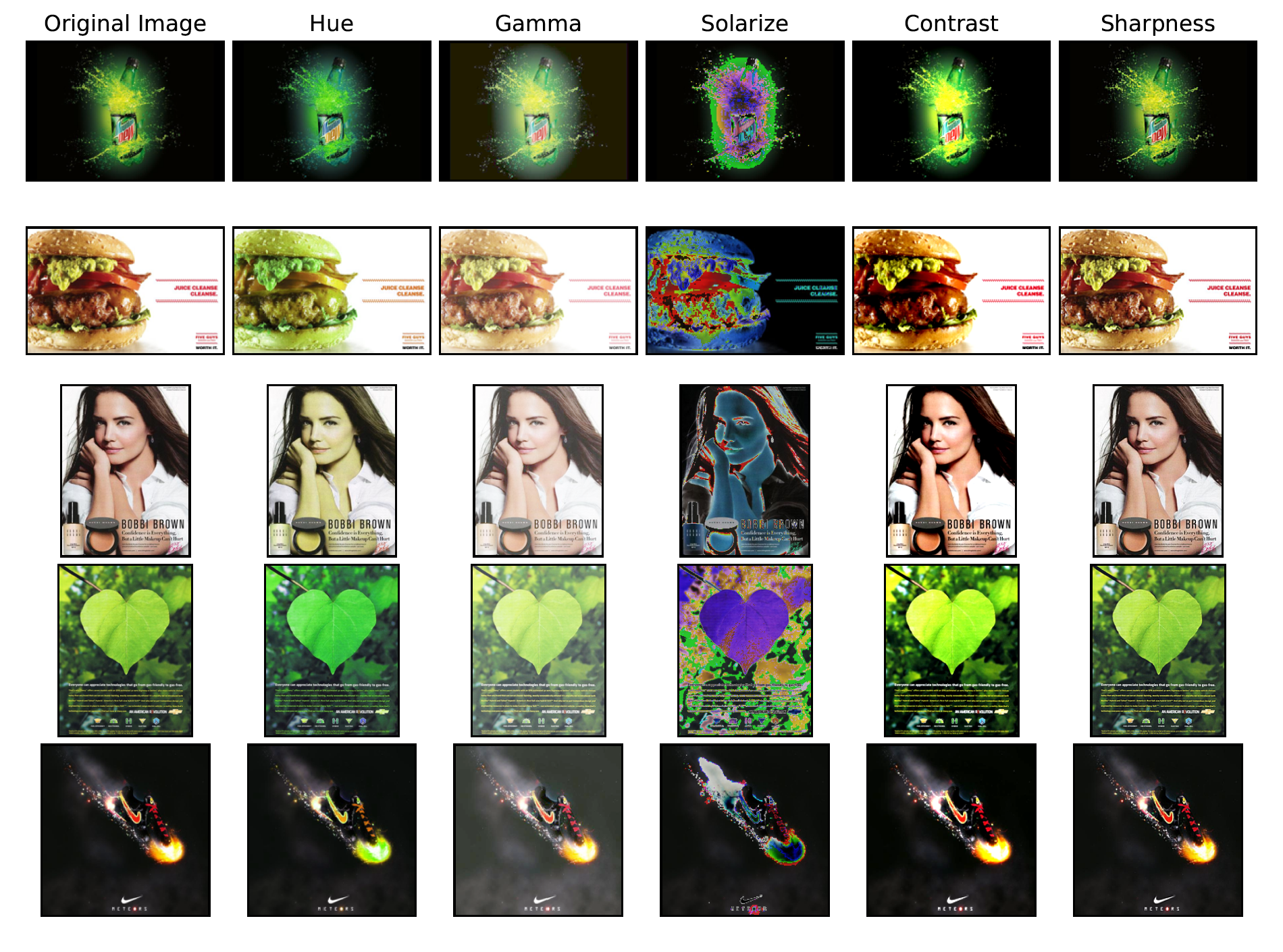
Even though brightness and contrast change show a potent outcome, a specific parameter cannot be kept for all images So, this processing approach has been handled in Data Augmentation section where functions like AutoContrast and AutoBrightness have been applied.
Histogram equalization, a popular technique for improving the contrast of images visibly failed to work for colored images. This technique was employed on a colored image which distorted colors and features such that it could not be considered as a viable preprocessing technique. The results are shown in the figure below where the image has been completely distorted in it’s entirety and is difficult for any feature to be mapped.

C. Data Augmentation Techniques
Data augmentation plays a crucial role in the training of deep learning models as they aren’t able to converge the network to an optimal solution if the size of training data is small because of the huge number of parameters needed to be tuned by the learning algorithm. It requires enormous amounts of data merely because of the fact that the deep learning algorithms start off with a poor initial state where weights are completely random and then optimization occurs using some gradient based optimization algorithm.
There are various ways to augment data using the PyTorch library such as RandomHorizontalFlip, RandomAdjustSharpness, etc that produce images with any random factor while training the network. Data augmentation also helps in creating images that may be a possible in the real world but are not depicted in the dataset properly. For example, a coffee mug might be perfectly straight in one image but it could be a tilted by 15 degrees in another image so RandomRotation helps generate such images. Some of the data augmentation techniques can be seen in the figure below which are RandomHorizontalFlip, RandomRotation and ColorJitter respectively.


D. Architectures
Different backbone architectures were chosen to ensure that different types of Convolution blocks were tested for the advertisement data. Resnet-50, MobileNet V3 Large and EfficientNet B3 were chosen finally with the selection criterias including number of parameters and GFLOPS, total training and evaluation time, and the top 5 classification accuracy on the ImageNet 1K benchmark dataset.
| Architecture | Params (Mil.) | Layers | GFLOPS | Imagenet Acc. |
|---|---|---|---|---|
| MobileNet V3 Large | 5.5 | 18 | 8.7 | 92.57 |
| EfficientNet B3 | 12.2 | 29 | 1.83 | 96.05 |
| Resnet-50 | 25.6 | 50 | 4.09 | 95.43 |
Results
First, training data with labels that were low in count were removed. Out of the 30 available labels, only the top 20 were chosen. Next, images where the label was categorised by only one person was discarded as it was observed that many of these images were incorrectly labeled.
Then, the advertisement images were pre-processed using the bilateral filter described above before resizing them to the size - 384 * 384. The data was split into train, test and validation set in the 0.6:0.2:0.2 ratio and was stored in separate directories according to the defined PyTorch dataloader.
The dataset used in this study presented the the multiclass, multilabel classification problem. Thus, to make the model predict multiple labels, a sigmoid layer had to be added before the loss function to get 0 or 1 prediction for all the classes of the data. To achieve this, the BCEWITHLOGITSLOSS function of PyTorch was used as it combines the Sigmoid layer and the binary cross entropy loss function in one single class. This makes theses operations more numerically stable than their separate counterparts.
The pre-trained weights were chosen to be the IMAGENET1K V2 weights and only the last classification layer was fine-tuned. The rationale behind performing this type of shallow-tuning was that the Imagenet data is very similar to the advertisement images in our dataset. Additionally, the size of the selected dataset is small so deep-tuning might not work well.

Training Results
| Model | F1 Score | Time | F1 epochs | Loss Epochs |
|---|---|---|---|---|
| MobileNet V3 Large | 0.168 | 80s | 50 | 98 |
| EfficientNet B3 | 0.189 | 153s | 5 | 90 |
| Resnet-50 | 0.179 | 50s | 10 | 0 |
It is clear that going from a smaller architecture to a bigger architecture, makes the model start to overfit earlier. The MobileNet model took the most number of epochs to reach the minima. The EfficientNet model performs the best for our dataset.
However, all three models performed poorly. This shows that the compound scaling of EfficientNet gives good results for the advertisement dataset. The reason for poor performance overall could be due to a number of reasons. The dataset had a high number of classes but the number of examples per class was very low.
Moreover, there was a high class imbalance problem. After looking at the images and the labels more closely, it was noticed that many images were poorly labeled and the labels contained quite a few synonyms.
The best model which in this case was the EfficientNet B3 model was used to do further analysis like visualizing the trained filters and using Grad-CAM to understand which areas of the image the model focused on to generate the predictions.
Observations

Looking at the figure above for it can be seen that the MobileNet architecture was the fastest to train per epoch. It took less time per epoch but, if number of epochs required to converge is considered, it does not train the fastest.
The lowest validation set loss for ResNet was at epoch 0. This means that the model started overfitting right after the first epoch in terms of the loss. However, it took 10 epochs to converge on the F1 score.
EfficientNet model performed the best in terms of the overall F1 score on the test set. Another surprising observation is that the EfficientNet model takes the longest to train per epoch even though the number of trainable parameters is nowhere close to ResNet but still it was chosen to plot the confusion matrix.
In the above figure, it can also be seen that the model classifies the labels Fashionable, Feminine, and Eager the best which are the classes that have the most number of training examples. This shows that if we increase the training dataset size, the models could improve a lot.
Grad-CAM Visualizations
As the EfficientNet B3 model produced the best F1 score on the test set, it was used to generate the GradCAM visualizations to understand the model output. The filters of the first layer have been visualized in the figure below.

We can see from the above figure that in the first layer of the network the model identifies prominent edges of the image. We can confirm this by looking at the filters of the first layer. Most of the filters look like they identify edges and corners.


In the middle layer of the network, the model is looking at many different features but isn’t looking at the most relavant features for that label.
And lastly, in the final layer of the network, the model looks only at the relavant features of the image depending on the current label. For example, here it is focusing on the player playing football for the ’Active’ label.
Conclusion
Visually looking at the gradcam visualizations and the predictions it is clear that the model is performing much better than what the F1 scores show.
The low performance of the models in this study can be attributed to the low quality of the labels along with a lack of available training data. Even though the convolutional layers of the EfficientNet model were not fine-tuned, it was observed that the model could find relavant features in the image depending on the label.
This shows that transfer learning is a powerful tool to train models and reduce turn-around times. Transfer learning enables the use of deep learning models even when the amount of available data is very less.
Acknowledgements & Feedback
I am grateful to have worked alongside Rohan Chopra who has helped me understand the essence of data pipeline generation, segregating tasks into workable components and to transform just jupyter notebooks into workable projects.
His profound understanding of machine learning concepts, algorithms, and techniques have greatly enhanced my interpretations and ability to tackle complex problems. He has consistently provided insightful feedback, constructive criticism, and practical suggestions, which have significantly improved the quality of our work together.
I would also love to receive suggestions or any feedback for this writing. It has been written as per my understanding and the learnings I kindled during my journey. I hope you find it useful and easy to understand.