Credit Risk Modelling
May 15, 2023
Financial institutions use credit risk analysis models to determine the probability of default of a potential credit borrower. If the lender fails to detect the credit risk in advance, it exposes them to the risk of default and loss of funds. Therefore, companies use models that provide information in respect to the riskiness or the level of a borrower’s credit risk at any particular time. Lenders rely on the validation provided by credit risk analysis models to make key lending decisions on whether or not to extend credit to the borrower and the credit to be charged.
Even though the results of these models are binary, that whether a person is risky or not but the outcomes are actually probabilitic values. These values determine the probability of a person being risky or not. The threshold value is set by the financial institution and the model is trained to predict the probability of a person being is a spectrum of being risky that is low to high.

Modelling Workflow
As the defaulters are a small percentage of the total population, the data becomes is highly imbalanced in these situations. This writing investigates the use of data under-sampling and oversampling techniques for resolving this class imbalance, the development of different classification machine learning models, and methodologies for comparing and evaluating these models. The code for this flow can be seen in the Github repo. The repository is kept private because of plagiarism reasons.

Data Preprocessing
Data preprocedding is a crucial part of building any machine learning model. The data can be skewed and can have outliers. So, the data is preprocessed to remove any missing values, outliers, or imbalance in dataser etc.
Missing Values
Missing values can be handled in various ways but the methods depends on the type of feature. The features can be continous or categorical. If the missing values occur in a continous feature then it can be replaced by the mean of the feature or by using some imputation techniques. If the missing values occur in a categorical feature then it can be replaced by making a seperate category for the missing values called as "Unknown". Unnecessary features or non-informative features can be dropped from the dataset. Another method to handle missing values can be to predict the missing values using some machine learning model (linear regression).
Encoding Categorical Features
One-hot encoding technique is used to encode categorical features into simple binary vectors of 1s and 0s, called ‘dummies’. The categorical features are then replaced by their ‘dummies’ in the dataset. This is done to avoid the model from misinterpreting the categorical features as numerical values.
Feature Scaling
Feature scaling is the process of normalising the range of features in a dataset. It is performed to ensure that all the features are on the same scale. The features can be on different scales and algorithms can interpret the values of features with higher scales as more important than the features with lower scales. This can be avoided by scaling the features to the same range by Normalisation, also known as min-max scaling, a scaling technique whereby the values in a column are shifted so that they are bounded between a fixed range of 0 and 1.
On the other hand, standardisation or Z-score normalisation is another scaling technique whereby the values in a column are rescaled so that they demonstrate the properties of a standard Gaussian distribution, that is mean = 0 and variance = 1. StandardScaler can be used to re-scale the numerical features in the dataset, in a way that the new distribution will have mean of 0 and standard deviation of 1.
EDA (Exploratory Data Analysis)
One must perform EDA to analyse the patterns present in the data which will make sure that the credits limits are not rejected for the applicants capable of repaying and to identigy outliers. When the company receives a credit application, the company has the rights for setting credit limit approval based on the applicant’s profile. These two types of risks are associated with the bank’s or company’s decision:
• If the aspirant is likely to repay the credit, then not approving the credit limit tends in a business loss to the company.
• If the a is aspirant not likely to repay the credit, i.e. he/she is likely to default/fraud, then approving the credit limits may lead to a financial loss for the company.

Data Balancing
The data is highly imbalanced as the defaulters are a small percentage of the total population. The data can be balanced using the following re-sampling techniques:
• Random Under-Sampling: Randomly select observations from the majority class to delete until the majority and minority class instances are balanced.
• Random Over-Sampling: Randomly duplicate observations from the minority class to increase the number of instances in the minority class.
• SMOTE (Synthetic Minority Oversampling Technique): SMOTE works by selecting examples that are close in the feature space, drawing a line between the examples in the feature space and drawing a new sample at a point along that line.
• NearMiss: NearMiss is an under-sampling technique that randomly eliminates examples from the majority class that are near the decision boundary using the k-nearest neighbors algorithm.
Perhaps, changing the performance metric can also help in understanding the data. The performance metric can be changed from accuracy leading to accuracy paradox where the accuracy measures tell the story that you have excellent accuracy (such as 90%), but the accuracy is only reflecting the underlying class distribution to F1-score or ROC-AUC curves/score.

And, lastly, the model can understand imbalanced dataset by cost-senstive learning. It is a machine learning paradigm for classification problems where the cost of misclassification is not the same for all the classes. The cost-sensitive learning can be implemented by using cost-sensitive learning algorithms such as:
• Penalized-SVM: Penalized-SVM is a cost-sensitive learning technique that penalizes the misclassification of the minority class by adding a cost term to the SVM objective function.
• Penalized-LR: Penalized-LR is a cost-sensitive learning technique that penalizes the misclassification of the minority class by adding a cost term to the LR objective function.
Evaluation Metrics
The below stated techniques are better suited for evaluating model in this case:
• Precision: answers the question, how many values belong to Actual positive out of the total positive predicted by model.
• Recall: answers the question, out of total positives, how many are predicted as positive by model.
• F1-score: Harmonic mean of Precision and Recall
• ROC Curve: summarizes trade-off between the true positive rate and false positive rate for a model using different probability thresholds. Higher area under the curve means a better model.
• Precision-Recall Curve: summarizes trade-off between Precision and Recall for a model using different probability thresholds. Higher the area under the curve means better the model.
To detect model overfitting, the models’ training and testing performance are evaluated using the metrics listed above. If the model’s training performance scores are higher than its testing performance scores, it is overfitting.
Model Building
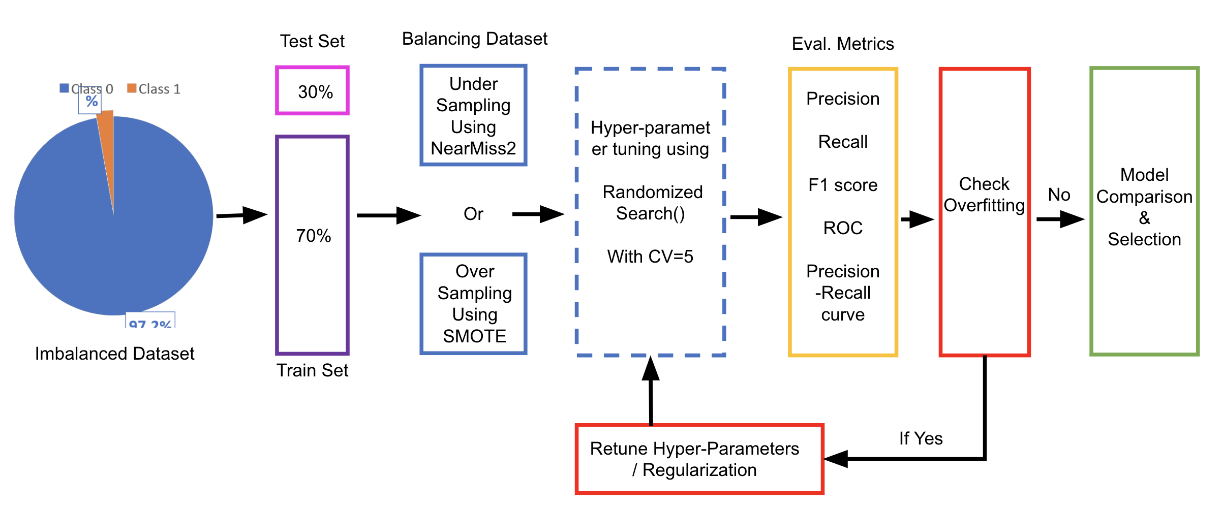
The dataset could be divided into training and testing sets using a 70:30 ratio. The training set can then be used for hyperparameter tuning the model as well. The training set can be fed into RandomisedSearch Cross validation with 5 folds. Due to 5-Fold cross validation, the training set is divided into 5 folds, for each unique fold 1 sub-dataset becomes a validation set and the remaining 4 become the training sets. These training and validation sets can then be used for hyperparameter tuning and model assessment.
RandomisedSearch can be used for hyperparameter tuning. Unlike GridSearch, which searches through all potential hyperparameter combinations, RandomisedSearch only explores a restricted collection of randomly picked hyperparameters, thus decreasing the search space and lowering the computing cost.
Experimentation (1)
Firstly, the models must be for binary credit default classification that are directly trained on the imbalanced dataset. In this case no data balancing strategy should used for balancing the dataset prior to training the model. One can use any machine learning model for this purpose namely, Logistic Regression, Random Forest, XGBoost, LightGBM.
| ML Model | Class | Performance | ||||
|---|---|---|---|---|---|---|
| Precision | Recall | F1 | ROC | Precision-Recall Curve | ||
| Random Forest | 0 | 0.98 |
1.00 |
0.99 |
0.5 |
0.51 |
| 1 | 0 | 0 | 0 | |||
| XGBoost | 0 | 0.98 |
1.00 |
0.99 |
0.5 |
0.51 |
| 1 | 0 | 0 | 0 | |||
| LightGBM | 0 | 0.98 |
1.00 |
0.99 |
0.5 |
0.51 |
| 1 | 0 | 0 | 0 |
All three models provide superior accuracy, recall, and f1 scores for the majority class (0) but do not perform well on the minority class (1). The same is also confirmed by the model’s poor ROC Area under the curve score and Precision-Recall area under the curve scores as well. This is due to the fact that the models are trained on an imbalanced dataset and are biased towards the majority class.
Experimentation (2)
For the second experiment, one can train models after performing under-sampling. In under-sampling the size of the majority class is reduced to match that of the minority class. In this experiment Near-miss 2 under sampling algorithm can be used for balancing the dataset. The algorithm works by selecting those samples of the majority class that have the smallest distance to the ‘k’ farthest samples of minority class.
| ML Model | Class | Performance | ||||
|---|---|---|---|---|---|---|
| Precision | Recall | F1 | ROC | Precision-Recall Curve | ||
| Random Forest | 0 | 0.86 |
0.98 |
0.91 |
0.90 |
0.94 |
| 1 | 0.97 |
0.83 |
0.89 |
|||
| XGBoost | 0 | 0.87 |
0.98 |
0.92 |
0.91 |
0.95 |
| 1 | 0.98 |
0.85 |
0.91 |
|||
| LightGBM | 0 | 0.86 |
0.98 |
0.92 |
0.90 |
0.943 |
| 1 | 0.98 |
0.83 |
0.90 |
It is clear that, when compared to the baseline models, the performance of all three modes has improved across all the metrics. In this scenario, the XGBoost model is the best of the three since it not only has the highest Precision, Recall, and F1 scores, but it also has a larger ROC Area under the curve score and Precision-Recall Area under the curve score as well.
Experimentation (3)
For the last experiment, one can train models after performing over-sampling. In this experiment, SMOTE oversampling algorithm can used for balancing the dataset. SMOTE oversamples the minority class by first taking a subset of data from the minority class as an example and then creating new synthetic similar instances which are then added to the original dataset.
| ML Model | Class | Performance | ||||
|---|---|---|---|---|---|---|
| Precision | Recall | F1 | ROC | Precision-Recall Curve | ||
| Random Forest | 0 | 0.93 |
0.93 |
0.93 |
0.93 |
0.947 |
| 1 | 0.93 |
0.93 |
0.93 |
|||
| XGBoost | 0 | 0.98 |
0.99 |
0.99 |
0.985 |
0.991 |
| 1 | 0.99 |
0.98 |
0.99 |
|||
| LightGBM | 0 | 0.97 |
1.00 |
0.98 |
0.981 |
0.989 |
| 1 | 0.99 |
0.97 |
0.98 |
After training the models on the oversampled data, the performance of all three improved across all when compared to the baseline models. In this situation, the performance of the three models outperforms their performance on under sampled data. In this case as well the XGBoost model is the best of the three since it not only has the highest Precision, Recall, and F1 scores, but it also has a larger ROC Area under the curve score and Precision-Recall Area under the curve score as well.
Conclusion
• From the above experiments it can be seen that balancing the dataset using either an under or over sampling strategy and then training the model on the balanced data considerably improves the classification model’s performance.
• The models’ performance is substantially greater when trained on balanced data using oversampling as opposed to undersampling Although all three machine learning models give similar performance, the XGBoost-based model outperforms the others in both oversampled and undersampled scenarios.
• The XGBoost model has the highest Precision, Recall, and F1 scores, as well as the largest ROC Area under the curve score and Precision-Recall Area under the curve score.
Acknowledgements & Feedback
I would love to receive suggestions or any feedback for this writing. It has been written as per my understanding and the learnings I kindled during my journey. I hope you find it useful and easy to understand.